Quantitative Measurement of the Phase Error for a Simple and Rapid
Phase-Unwrapping Algorithm
G.S. Sobering#+, Y. Shiferaw*, P. van Gelderen*, C.T.W. Moonen*
#Laboratory of Diagnostic Radiology Research
*In Vivo NMR Research Center
NIH, Bethesda, MD, USA
+Present address: GE Medical Systems, Milwaukee, WI, USA
Poster at 1995 SMR Annual Meeting
Introduction:
There are many applications which require the creation
of MR phase images. In our lab, we are particularly
interested in obtaining maps of the water frequency to
determine static B0 for use as a priori information in
spectroscopic imaging analysis and for measuring
temperature in vivo via the water chemical shift.
When computing phase maps from complex-valued MR
images, the range of phase angles often exceeds ±2 radians
across the image. This causes artifactual discontinuities (so-
called "wraps") in the image where the phase angle jumps
from +
 to -
to - , or -
 to +
to + . A powerful and simple method
for calculating the relative phase between any two points in a
complex-valued array (image or 3D volume) is to sum the
incremental angular differences between neighboring voxels
along a path connecting the two points [1]. The
"unwrapping" problem is thus reduced to selecting an
algorithm that connects all the voxels in the object to a single
reference voxel.
In the ideal case, the phase determined by this
unwrapping procedure is path independent. However, in real
data, noise and regions of low signal can cause incorrect
results. Many algorithms have been developed to address
this problem [2-5]. The computational requirements of
some of these algorithms are quite steep, especially for 3D
data-sets.
In this abstract, we describe the analysis of phase maps
generated using a variety of simple path algorithms. These
maps demonstrate the insensitivity of this technique to the
choice of path selection algorithm for typical MR data. This
implies that simple (and rapid) path creation algorithms,
using image magnitude to identify "bad" voxels, may be used
successfully. Here, one such algorithm is described and
evaluated in detail.
Experimental:
Images were collected with a variety of gradient echo
pulse sequences on a 1.5T clinical scanner. Data from both
phantom and in vivo studies was analyzed.
Complex images were computed using standard Fourier
reconstruction. Static phase effects were removed by
dividing an image acquired at long TE by an otherwise
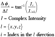
identical short TE image. The spatial derivatives
(differences) of the phase maps were computed using the
same division process:

This method of calculating
 Ø/
Ø/ l
has the advantage that it
directly evaluates the difference phase angle between the two
locations, even if they happen to be on either side of ±
l
has the advantage that it
directly evaluates the difference phase angle between the two
locations, even if they happen to be on either side of ± phase-wrap. This means that phase-wraps present in the
original image do not affect the
 Ø/
Ø/ l
values, unlike the
direct method:

Two path algorithms were used to generate maps for this
analysis. The first is a very simple rectilinear algorithm,
which is presented not as a practical method, but to
demonstrate the insensitivity of this class of techniques to
non-optimal path choice. In this algorithm, the paths follow
the imaging grid axes. For example, in a 2D image, one path
between (15,10) and (20,25) would move from (15,10)
across to (20,10), and then up to (20,25). For 2D images
there are two possible paths (denoted: xy and yx) between
any two points, and for 3D volumes there are six (xyz, yzx,
zxy, yxz, xzy, zyx). In practice, this algorithm has many
disadvantages. Most troubling is that many objects cannot be
fully unwrapped, because all the rectilinear paths connecting
some points inside the object traverse the exterior region.
The second path algorithm is more optimal and robust.
It is based on a standard seeded region growing algorithm.
The algorithm is started with a single-voxel region at the
reference point. At every iteration:
- The list of voxels on the exterior boundry of the region
is sorted by magnitude (highest to lowest).
- For each voxel on the list, the phase of all nearest
neighbor voxels that have not already been visited (or
been previously marked as below the intensity
threshold) is computed using the appropriate
 Ø/
Ø/ l
map. The neighbor voxels are marked as visited, and
added to the list of boundry voxels for the next
iteration.
Iteration continues until the "next iteration boundry
voxels" list is empty. This algorithm has a number of
advantages:
- It is computationally simple and fast.
- The region will grow around inclusions of "bad" pixels
inside the object.
- The selected path is locally optimized in the sense that
given an unvisited voxel with multiple visited nearest-
neighbors, the path from the highest magnitude
neighbor will be used.
Analysis:
In order to evaluate the errors in these methods, phase
maps were produced using the two algorithms described
above. This gave seven maps produced using very different
paths (the six possible rectilinear paths for a 3D volume, and
the one from the region-growing method). The differences
between the seven phase values were compared by calculating
the standard deviation and maximum difference for every
point in a large VOI placed inside the object (phantom, brain,
etc.). Results for two typical data-sets are shown below.
The phantom data was acquired using a two sequential
3D volume FLASH acquisitions with TE1/TE2/TR of
10/30/41ms. SNR in the long-TE image was 60. The in vivo
data was acquired from a human brain study using a 3D
volume multi-echo FLASH sequence. The first and fourth
echoes were used in the analysis, giving a TE1/TE2/TR of
10/40/55ms. SNR in the long-TE image was ca. 100.
                      Phantom            Brain
                  --------------     --------------
             s    4.8e-8 radians     3.2e-7 radians
          max.    3.6e-7 radians     1.9e-6 radians
Conclusions:
The extremely small errors measured between these
methods indicate that relatively computationally simple and
fast routines can successfully unwrap phase maps from
typical MR images. The choice of path algorithm is not
critical, as long as obviously low intensity regions are
avoided. The region-growing algorithm presented here is
robust and can successfully unwrap most MR images, even in
the presence of large phase changes across the object.
References:
- K. Ito, Appl. Opt., 21, 247 (1982)
- D. Ghiglia, et al., J. Opt. Soc. Am. A 4, 267 (1987)
- M. Hedley, D. Rosenfeld, SMRM 8th Annual Meeting, 920 (1989)
- G. Scott, M.L.G Joy, SMRM 10th Annual Meeting, 747 (1991)
- M. Hedley, D. Rosenfeld, Magn. Reson. Med., 24, 177 (1992)
 radians
across the image. This causes artifactual discontinuities (so-
called "wraps") in the image where the phase angle jumps
from +
 to -
to - , or -
 to +
to + . A powerful and simple method
for calculating the relative phase between any two points in a
complex-valued array (image or 3D volume) is to sum the
incremental angular differences between neighboring voxels
along a path connecting the two points [1]. The
"unwrapping" problem is thus reduced to selecting an
algorithm that connects all the voxels in the object to a single
reference voxel.
 Ø/
Ø/